Closeness Centrality
We all have an intuitive understanding when we say a home, an office, or a store is "centrally located." Closeness Centrality provides a precise measure of how "centrally located" a vertex is. The steps below show the steps for one vertex v:
| Step | Mathematical Formula |
|---|---|
1. Compute the average distance from vertex v to every other vertex: |
\(d_{avg}(v) = \sum_{u \ne v} dist(v,u)/(n-1)\) |
2. Invert the average distance, so we have average closeness of v: |
\(CC(v) = 1/d_{avg}(v)\) |
TigerGraph’s closeness centrality algorithm uses multi-source breadth-first search (MS-BFS) to traverse the graph and calculate the sum of a vertex’s distance to every other vertex in the graph, which vastly improves the performance of the algorithm. The algorithm’s implementation of MS-BFS is based on the paper The More the Merrier: Efficient Multi-source Graph Traversal by Then et al.
|
This algorithm query employs a subquery called |
Specifications
tg_closeness_cent (SET<STRING> v_type, SET<STRING> e_type, INT max_hops=10,
  INT top_k=100, BOOL wf = TRUE, BOOL print_accum = True, STRING result_attr = "",
  STRING file_path = "", BOOL display_edges = FALSE)
Parameters
| Characteristic | Value |
|---|---|
Result |
Computes a Closeness Centrality value (FLOAT type) for each vertex. |
Required Input Parameters |
|
Result Size |
V = number of vertices |
Time Complexity |
O(E), E = number of edges. Parallel processing reduces the time needed for computation. |
Graph Types |
Directed or Undirected edges, Unweighted edges |
Example
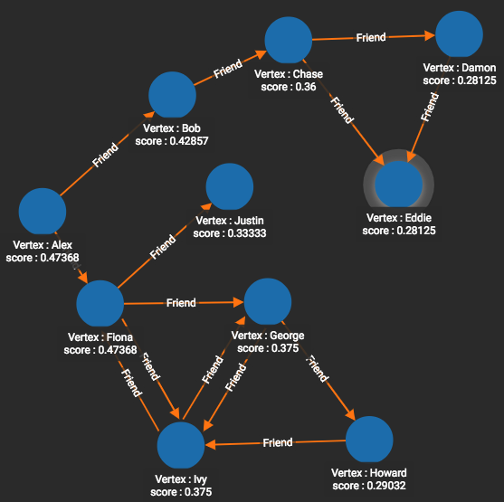
Closeness centrality can be measured for either directed edges (from v to others) or for undirected edges. Directed graphs may seem less intuitive, however, because if the distance from Alex to Bob is 1, it does not mean the distance from Bob to Alex is also 1.
For our example, we wanted to use the topology of the Likes graph, but to have undirected edges. We emulated an undirected graph by using both Friend and Also_Friend (reverse-direction) edges.
# Use _ for default values
RUN QUERY tg_closeness_cent(["Person"], ["Friend", "Also_Friend"], _, _,
_, _, _, _, _)